简体中文 | English | 旧版README | Old Version README


Log service is a cloud-native observation and analysis platform that provides large-scale, low-cost, and real-time platform services for Log, Metric, and Trace data. One-stop data collection, processing, analysis, alarm visualization, and delivery are provided to improve the digitization capabilities of R & D, O & M, operations, and security scenarios. Official documentation
this repository is an Alibaba Cloud log service Grafana data source plug-in. Before using this plug-in, you must use log service products and have at least one LogStore configured for collection.
The dependency Grafana version 8.0 and later. Grafana version 8.0 and later, use version 1.0.
download from Release . Go to the grafana plug-in directory and modify the configuration file. [plugins] node, set allow_loading_unsigned_plugins = aliyun-log-service-datasource , and then restart the grafana.
- mac
- Plug-In Directory:
/usr/local/var/lib/grafana/plugins - Configuration file location:
/usr/local/etc/grafana/grafana.ini - Restart command:
brew services restart grafana
- Plug-In Directory:
- YUM/RPM
- Plug-In Directory:
/var/lib/grafana/plugins - Configuration file location:
/etc/grafana/grafana.ini - Restart command:
systemctl restart grafana-server
- Plug-In Directory:
- .tar.gz
on the datasource page, add an SLS log-service-datasource data source. In the data source management panel, add a LogService data source. In the settings panel, set the Endpoint project for your log service endpoint ( endpoint can see it on the overview page of the project. For more information, see service entry ). For example, if your project is in the qingdao region, enter the Url cn-qingdao.log.aliyuncs.com . Set the Project and logstore as needed, and set the AccessId and AccessKeySecret. It is best to configure the accesskey of the sub-account. To ensure data security, the AK is saved and cleared without Echo.
3.2 Time series database configuration (using SLS plug-in, supports SQL query and combination operator query)
the time series library can also be configured as an SLS plug-in. With this access method, you can query the time series Library by SQL or by using the PromQL operator. For more information, see: description of time series query syntax ). The configuration method is the same as that in Section 1.1. Enter the name of the LogStore in the metricStore.
the SLS time series Library supports native Prometheus query, so you can directly use the native Prometheus plug-in to access the data source. Please refer to the following official documentation configure the data source. The URL of the log service MetricStore in the format **https://{project}. {sls-endpoint}/prometheus/{project}/{metricstore} **. Where _{sls-endpoint} _the Project of the region where the Endpoint is located. For more information, see service entry , _{project} _and _{metricstore} _replace the Project and Metricstore of the created Log service with the actual value. For example: https://sls-prometheus-test.cn-hangzhou.log.aliyuncs.com/prometheus/sls-prometheus-test/prometheus
From the perspective of best practices, you can add Prometheus data sources and SLS data sources to the time series database at the same time. You can use different statement query methods according to your personal habits. We recommend that you use SLS data sources in Variable (you can convert them to SLS dashboards)
in practice, the only recommended writing method is: ${var_name} .
Theoretically, Grafana supports three writing methods: $varname , ${var_name} , [[varname]] . However, if you do not add parentheses, the variable name range may be incorrectly identified, and the double-Middle plus sign will be gradually abandoned in the future. Reference source .
for most SLS DataSource, you can use SQL statements to query values as variables. Procedure:
- go to Grafana dashboard settings-Variables
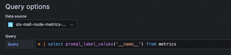
- select Query type, set Datasource to corresponding LogStore, and write query
- view the results in the Preview of values
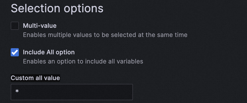
Generally, if you use it as a logstore filter, we recommend that you open it in practice. All Option and configure the Custom all value * .
In this way, Dashboard Query statement is written as follows: * and request_method: ${var} | select * from log you can select Variable and select all.


As mentioned in the configuration of SLS storage data sources, SLS time series libraries can be configured Prometheus either native or SLS plug-ins. If you use the SLS plug-in, you usually need to use the promql operator. For more information about the usage and syntax, see: overview of time series data query and analysis .
The following example shows how to obtain the names of all metrics in the time series database.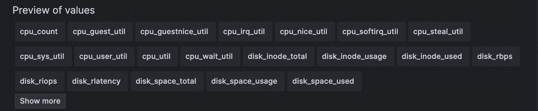
configure a Grafana time variable
| Name | Variable name, such as myinterval. The name is the variable used in your configuration. In this case, the myinterval. **$$myinterval **. |
|---|---|
| Type | Select **Interval **. |
| Label | Configure **time interval **. |
| Values | Configure **1 m, 10 m, 30 m, 1 h, 6 h, 12 h, 1d, 7d, 14d, 30d **. |
| Auto Option | Open **Auto Option **switch, other parameters remain the default configuration. |
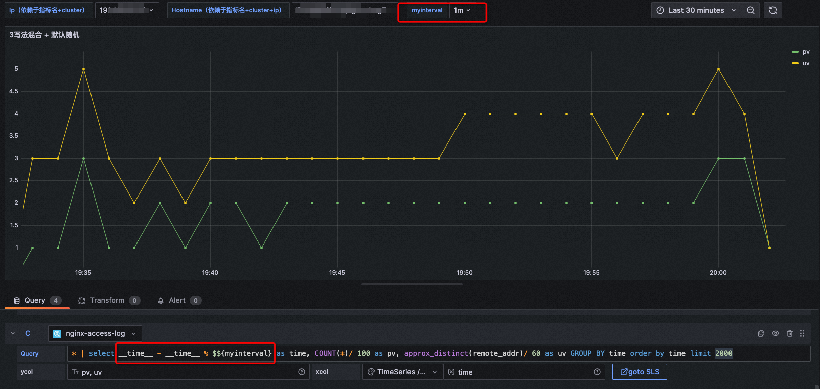
**Note: this time variable is different from Grafana variable in SLS. You need to add another variable before writing the normal variable. ****$ **to correctly convert Interval in SLS statements.
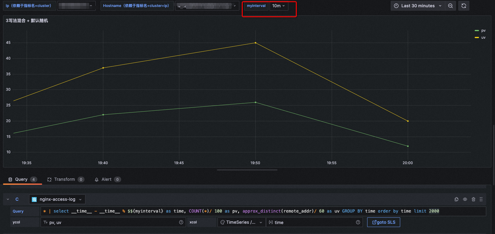
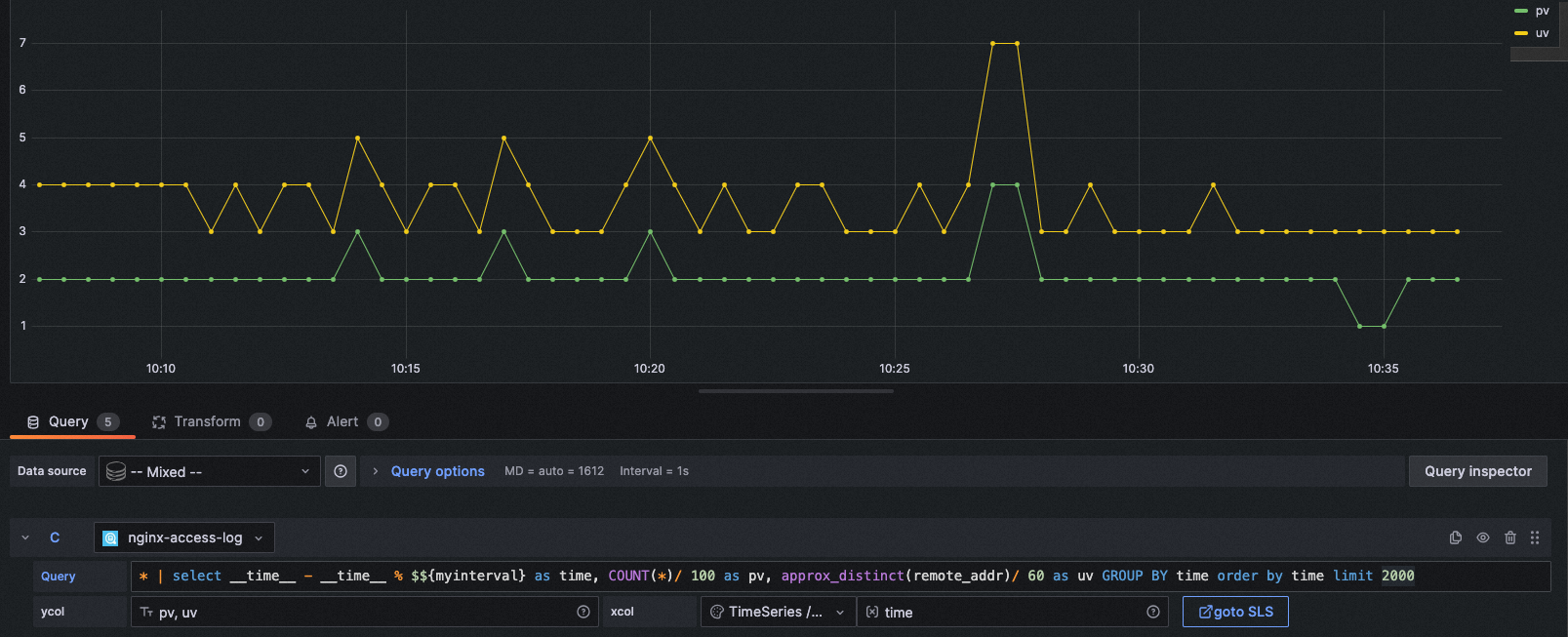
chartType: TimeSeries
xcol: time
ycol: pv, uv
query: * | select __time__ - __time__ % $${myinterval} as time, COUNT(*)/ 100 as pv, approx_distinct(remote_addr)/ 60 as uv GROUP BY time order by time limit 2000
In the configuration 1m when:
In the configuration 10m when:
When the time range of the dashboard is very long, this function can easily control the time hitting density.
xcol: stat
ycol: <Numeric column>, <Numeric column>
Note: If the required numeric column is a non-numeric column, it will be set to 0.
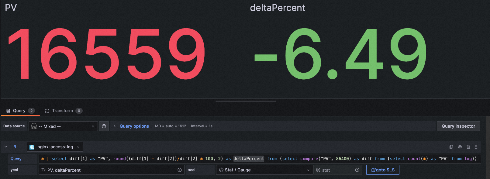
Example 1:
chartType: Stat
xcol: stat
ycol: PV, deltaPercent
query: * | select diff[1] as "PV", round((diff[1] - diff[2])/diff[2] * 100, 2) as deltaPercent from (select compare("PV", 86400) as diff from (select count(*) as "PV" from log))
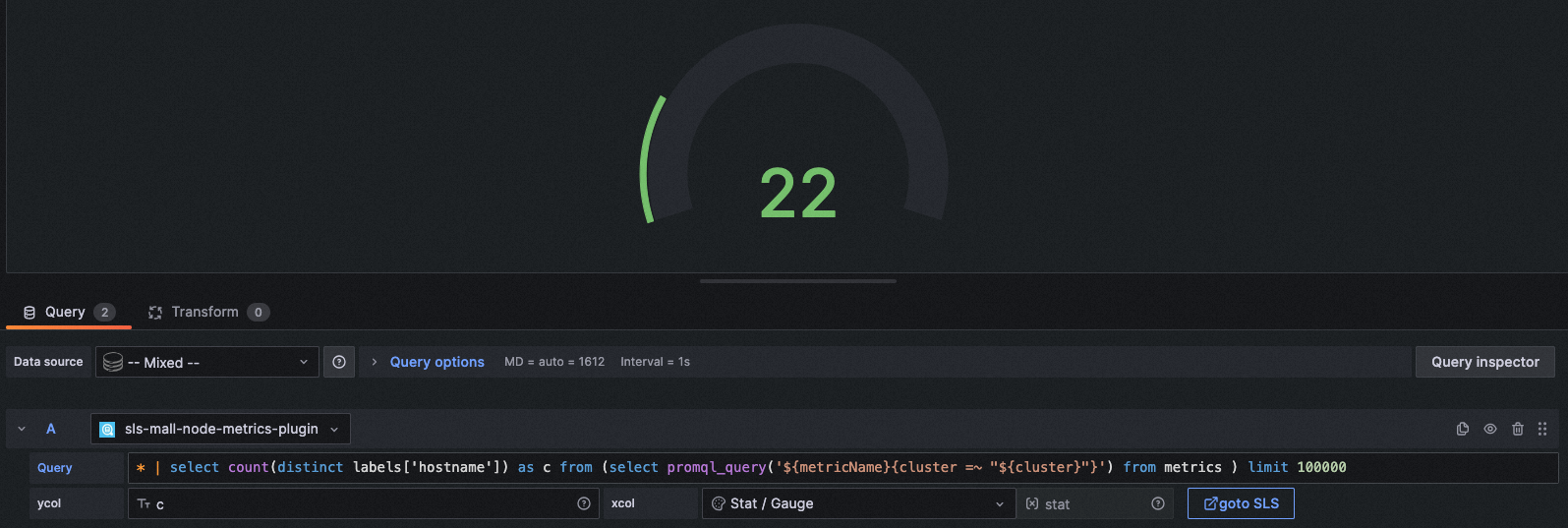
Example 2:
chartType: Gauge
xcol: stat
ycol: c
query: * | select count(distinct labels['hostname']) as c from (select promql_query('${metricName}{cluster =~ "${cluster}"}') from metrics ) limit 100000
Other scenarios:
online Graph scenarios can also be displayed as single-value graphs, but this writing method is not recommended.
xcol: pie
ycol: <Aggregate columns>, <Numeric column>
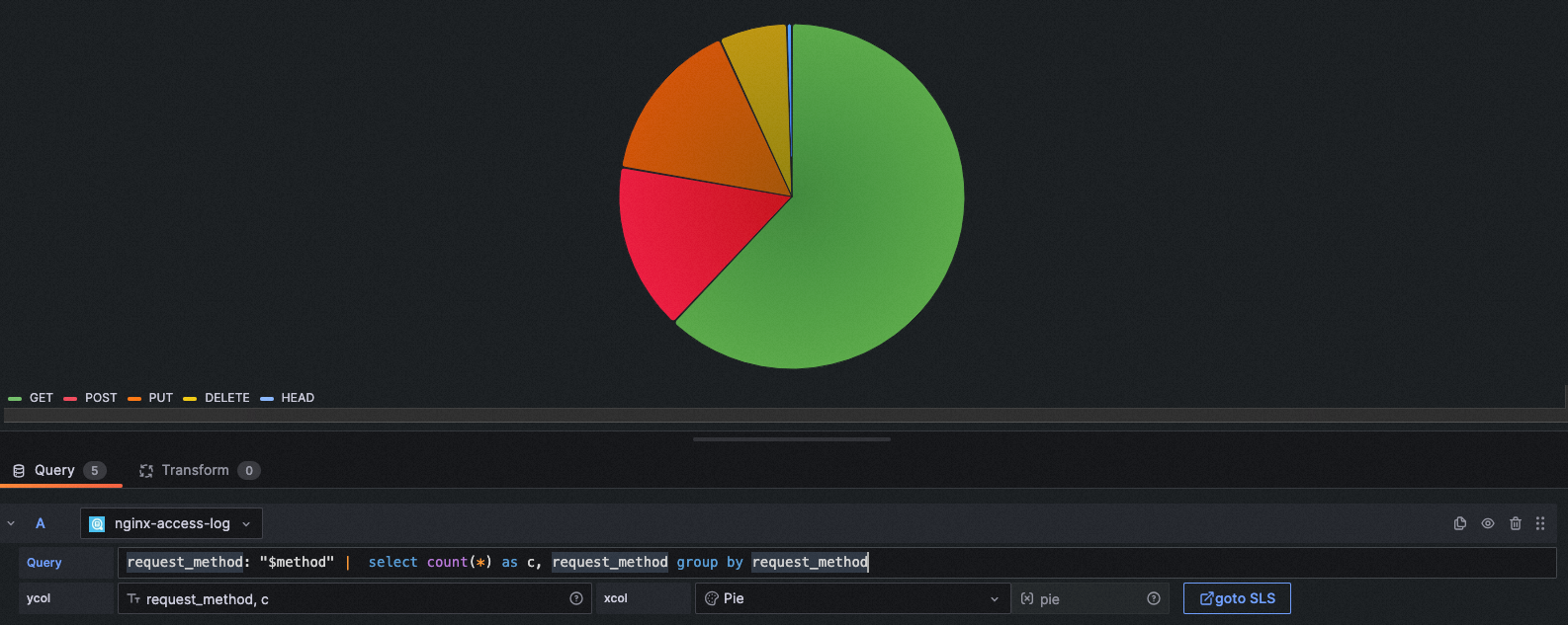
Example 1:
chartType: Pie
xcol: pie
ycol: request_method, c
query: request_method: "$method" |  select count(*) as c, request_method group by request_method
Example 2:
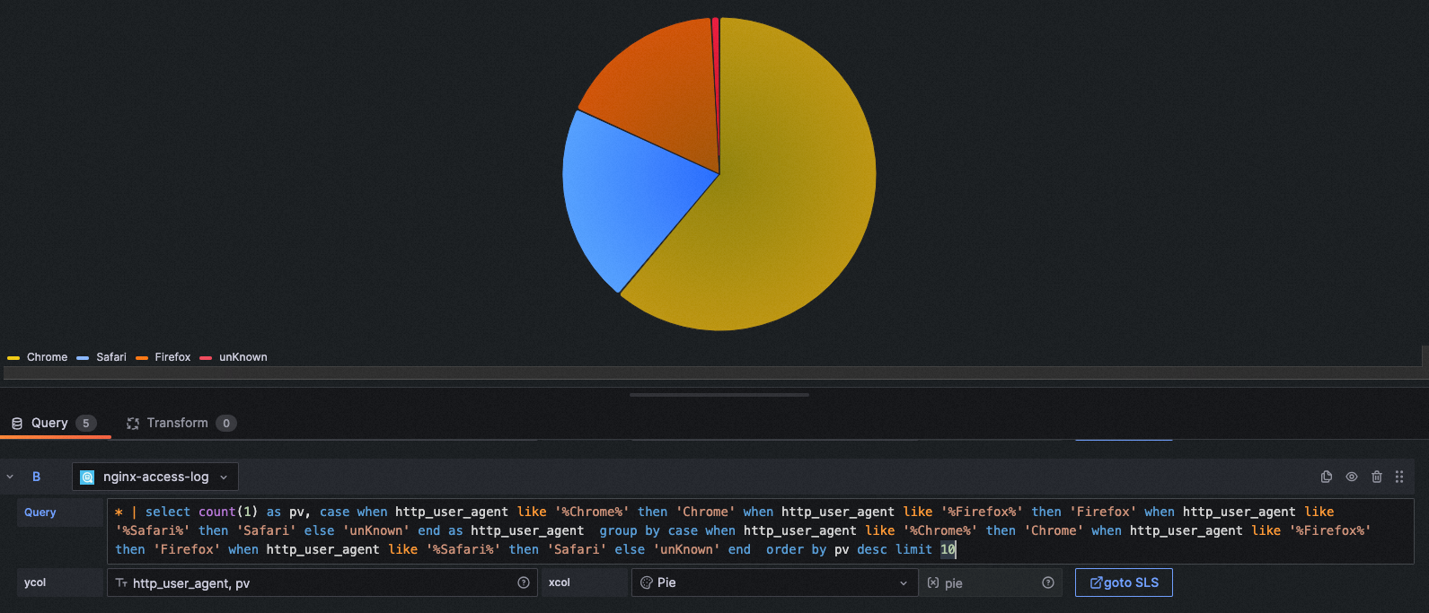
chartType: Pie
xcol: pie
ycol: http_user_agent, pv
query: * | select count(1) as pv, case when http_user_agent like '%Chrome%' then 'Chrome' when http_user_agent like '%Firefox%' then 'Firefox' when http_user_agent like '%Safari%' then 'Safari' else 'unKnown' end as http_user_agent  group by case when http_user_agent like '%Chrome%' then 'Chrome' when http_user_agent like '%Firefox%' then 'Firefox' when http_user_agent like '%Safari%' then 'Safari' else 'unKnown' end  order by pv desc limit 10
Other scenarios:
the Stat chart is also applicable to pie charts and can also show the effect.
chartType: Pie
xcol: stat
ycol: hostNameNum, ipNum
query: * | select count(distinct labels['hostname']) as hostNameNum, count(distinct labels['ip']) + 20 as ipNum from (select promql_query('${metricName}{cluster =~ ".*"}') from metrics ) limit 100000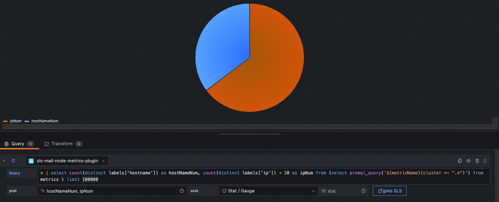
xcol: <Time column>
ycol: <Numeric column> [, <Numeric column>, ...](LogStore)<labels / Aggregate columns>#:#<Numeric column>(Write Time series Library or log aggregation)
Example 1:
chartType: Time series
xcol: time
ycol: pv, uv
query: * | select __time__ - __time__ % $${myinterval} as time, COUNT(*)/ 100 as pv, approx_distinct(remote_addr)/ 60 as uv GROUP BY time order by time limit 2000
Example 2:
chartType: Time series
xcol: time
ycol: labels#:#value
query: * | select time, * from (select promql_query_range('${metricName}') from metrics) limit 1000
Example 3:
you can also use SQL to customize time series labels.
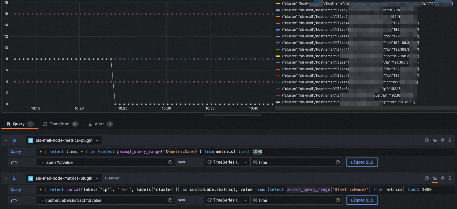
chartType: Time series
xcol: time
ycol: customLabelsExtract#:#value
query: * | select concat(labels['ip'], ' -> ', labels['cluster']) as customLabelsExtract, value from (select promql_query_range('${metricName}') from metrics) limit 1000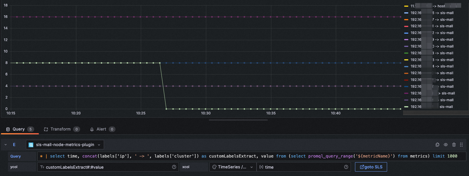
xcol: bar
ycol: <Aggregate columns>, <Numeric column> [, <Numeric column>, ...]
Example 1:
chartType: Bar
xcol: bar
ycol: host, pv, pv2, uv
query: * | select host, COUNT(*)+10 as pv, COUNT(*)+20 as pv2, approx_distinct(remote_addr) as uv GROUP BY host ORDER BY uv desc LIMIT 5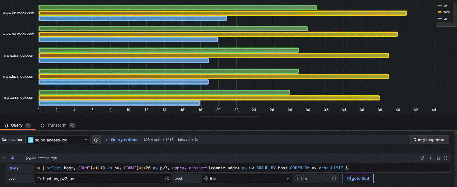
xcol: <empty>
ycol: <empty> or <Display Column> [, <Display Column>, ...]
Example 1:
chartType: Table
xcol:
ycol:
query: * | select __time__ - __time__ % 60 as time, COUNT(*)/ 100 as pv, approx_distinct(remote_addr)/ 60 as uv GROUP BY time order by time limit 2000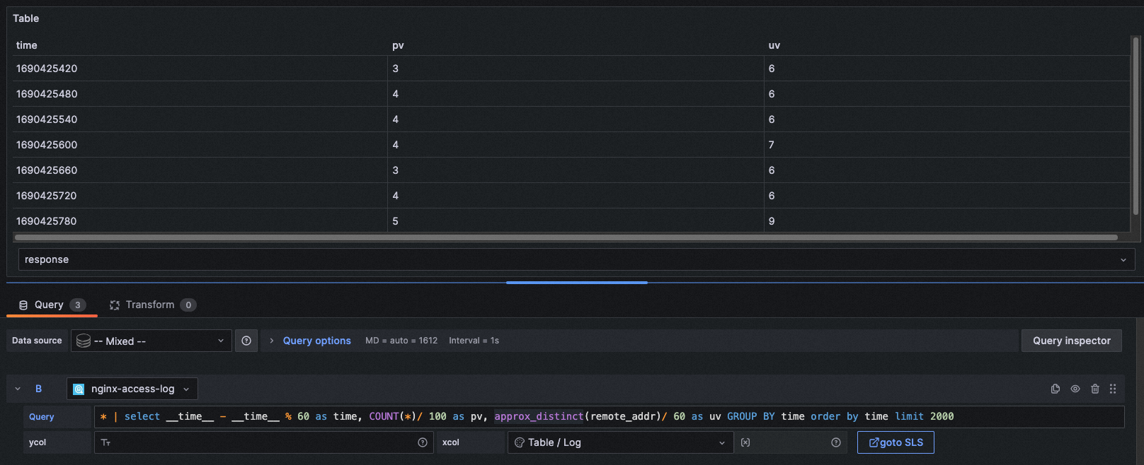
xcol: <空>
ycol: <空>
Example 1:
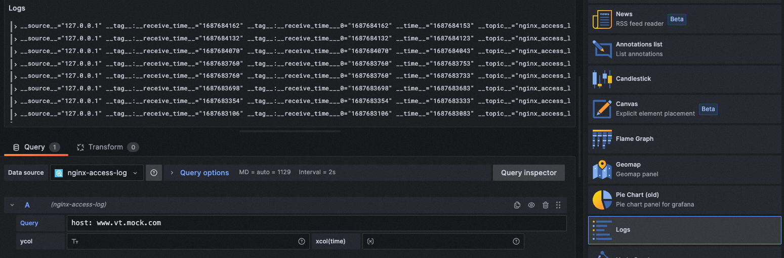
chartType: Logs
xcol:
ycol:
query: host: www.vt.mock.com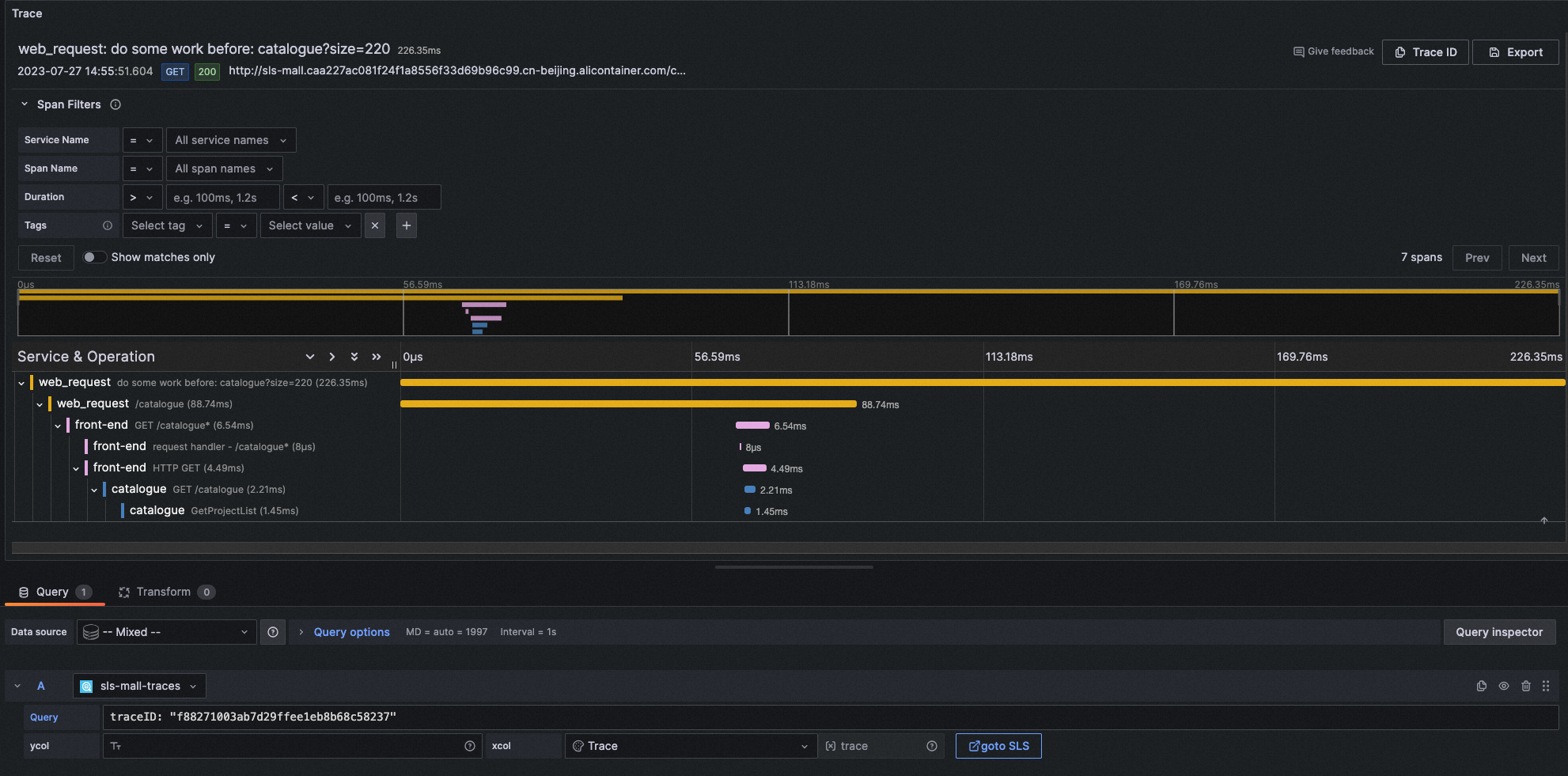
chartType: Traces
xcol: trace
ycol:
query: traceID: "f88271003ab7d29ffee1eb8b68c58237"
In this example, the Trace logstore is used. You need to use the Trace service in SLS. Log service supports native access to OpenTelemetry Trace data, and supports access to Trace data through other Trace systems. For more information, see: https://help.aliyun.com/document_detail/208894.html
in Grafana 10.0 and later versions, the span filtering function of Trace data is supported. If you are using a lower version Grafana, you can also customize the span filtering function in query filtering. For example:
traceID: "f88271003ab7d29ffee1eb8b68c58237" and resource.deployment.environment : "dev" and service : "web_request" and duration > 10
xcol: map
ycol: <Country column>, <Geographic location column>, <Numeric column>
Example 1:
chartType: GeoMap
xcol: map
ycol: country, geo, pv
query: * | select count(1) as pv ,geohash(ip_to_geo(arbitrary(remote_addr))) as geo,ip_to_country(remote_addr) as country  from log group by country having geo <>'' limit 1000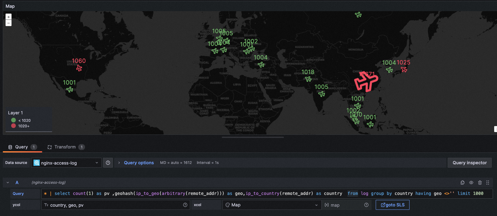
Note: This feature is only available SLS Grafana Plugin version 2.30 and later. You can jump to the SLS console at any time on the Explore and dashboard interfaces. You can also use the more powerful functions and flexible log retrieval of the SLS console.
Jump to the SLS console, with query and time information, without manual input.
This method is to jump directly to the SLS console without any configuration. However, you must log on to the SLS console with your browser. Otherwise, the login page will be displayed.

Procedure:
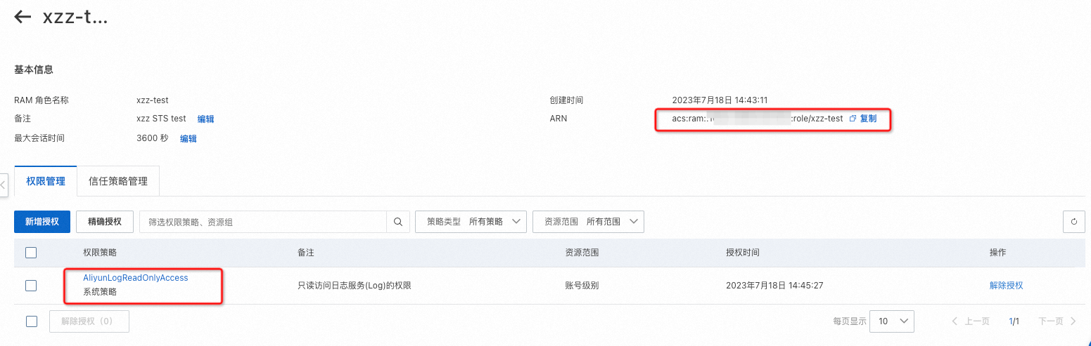
- access the RAM console https://ram.console.aliyun.com/roles/ , create a **_yes and only AliyunLogReadOnlyAccess _**the role of the policy. The recommended maximum session time is 3600 seconds. You can copy roleArn information in the basic information section.
- Access the RAM console authorization interface https://ram.console.aliyun.com/permissions to grant Grafana DataSource and AccessKey permissions to the user corresponding to the AliyunRAMReadOnlyAccess configured in the AliyunSTSAssumeRoleAccess. (Or change the Grafana DataSource and AccessKey configured by the AccessSecret. You must ensure that the user has this permission.)
- On the DataSource page, configure the roleArn.
- Return to the Explore interface again and try to gotoSLS the button to avoid STS redirection.

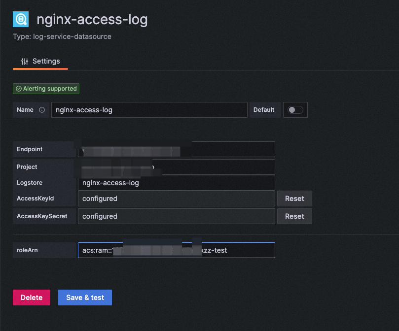
Note: If the configured roleArn is incorrect or the permission range is incorrect, the logon-free function will become invalid and will be redirected according to the general logic.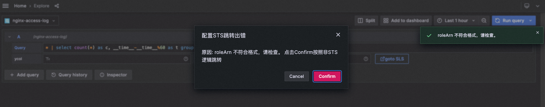
if STS redirection is configured, the following conditions must be met for permission security:
- the user corresponding to the DataSource of the configuration accessKey.
AliyunRAMReadOnlyAccesspermissions,AliyunSTSAssumeRoleAccesspermission - configure the DataSource of the roleArn. The policy must be **yes and only **
AliyunLogReadOnlyAccess
principle reference: embedded and shared in the console
If you configure no-logon redirection, be sure to check whether the data source involves sharing Grafana public access to the dashboard. If public access is involved, potential traffic costs may rise and potential log content may be exposed.
- check whether xcol and ycol are configured properly. For more information, see chapter 4.
- Leave xcol and ycol blank and check whether the data is correct in tabular form.
- Check whether the numeric column contains non-numeric characters or special characters.
- Check whether data is returned in the Query Inspector.
- Contact us to check this issue.
Check whether the SQL statement contains the date_format function. If yes, specify the following code in the pattern string:%Y-%m-%d %H:%i:%s
For example, the error statement is as follows:
* | SELECT date_format(date_trunc('minute', __time__), '%H:%i') AS time, COUNT(1) AS count, status GROUP BY time, status ORDER BY timeChange to:
* | SELECT date_format(date_trunc('minute', __time__), '%Y-%m-%d %H:%i:%s') AS time, COUNT(1) AS count, status GROUP BY time, status ORDER BY timeDingTalk Group