Consumer behavior prediction, based on Taobao data

0. Team Member

Name	Student ID	GitHub
Zhang Ping	1901212672	Parametric3
Xu Chenqi	1901212653	XuChenqi
Lin Haoru	1901212609	HalinaLin
Luo Chaojing	1901212618	crystallake27

1. Background

E-commerce has gradually become an essential part of our daily life. In 2019, China's online consumption accounted for more than 25% of total consumption. Under this situation, taking advantage of the big data generated by online transactions, we can analyze and reasonably predict consumer behavior.

Our team obtained Taobao's consumer behavior data from Tianchi, AliCloud, starting from November 18, 2014 to December 18, 2014. Based on that, we derived a series of other features which help interprete the consumer behaviors, and performed corresponding data preprocessing. After that, we comprehensively conducted LR, SVM, Decision Tree, Random Forest.

2. Data

Our data is from Tianchi, AliCloud, starting from November 18, 2014 to December 18, 2014. The original data includ two files. One is named tianchi_fresh_comp_train_user.csv, which is about all the users' bahaviors on all the items in that period, inclouding 6 basic indicators, user id, item id, behavior type (browse, collect, purchase, etc.), user geohash (location), item category and time.

Name	Meaning	Explain
user_id	the unique user identidication
item_id	the unique item identidication
behavior_type	the classification of user behavior	browing, collecting, adding into cart and purcahsing, corresponding to 1, 2, 3 and 4 respectively
user_geohash	the location of the user	can be null
item_category	the category of one certain item
time	time when behaving	precised to hour

For example, 141278390,282725298,1,95jnuqm,5027,2014-11-18 08.

The other file is named tianchi_fresh_comp_train_item.csv, which is about all the items, inclouding 3 basic indicators, item id, item geohash (location), item category.

Name	Meaning	Explain
item_id	the unique item identidication
item_geohash	the location of the item	can be null
item_category	the category of one certain item

For example, 117151719,96ulbnj,7350.

For detailed data, see our data in PKU Cloud.

3. Overall Analysis

3.1 Problem Type: Classification

'Prucahse' correspodning to '1', and 'Not Purchase' corresponding to '0'

Particularity of the problem:

1. The label is not just for one user or one item, but for one user-item pair (user, item), which influence the selection of training set and test set
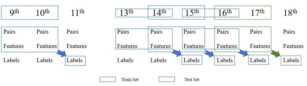
2. This is multi-period problem. For example, for one user-item pair, its label is derived from the bahevior of 18th, while its features are derived from days before 18th. That is because we can only the past to predict the future.

3.2 Days that really matter

Since we will use the information before 18th to predict the user behavior in 18th, the next question is how many days should be considered. Intuitively, the behavior one month ago definetely has nothing to do with whether the user will buy or not. So this actually a hyperparameter that we should decide first, and then find its best value through fine-tuning. Using $\Delta$ to denote it, and we let $\Delta$ = 2 at first. Later, we will also implement the same preprocessing and model on the datasets with $\Delta$ = 3 and 4 respectively.

3.3 Test Set

Three ways to choose test set:

1. All users and all items:
2. Users who have certain behaviors and the items that users has interactions with in the two days before :
3. For each user who was active before, only condider the items that he has interactions with:

Considering the handleable data size, we finally choose the third method, which also avoids the problem of sparse matrix at the same time.

3.4 Train Set

The basic rules all the same for train set. Two things to consider:

1. As customary, we set the ratio between the training set and the test set to be 4:1. So since we have choose (16, 17 → 18) as the test set (before '→', the features of test set; after '→', the labels of the test set), we need to choose another four groups.
2. If we count back from 18th, the abnormal comsumption in 12th, December will distrurb our model greatly, so we need to skip that when choose the train set.

The overall process is shown below, and related data that has been processed is in our Data folder.

4. Feature Generating

All the features can be dicided into two levels:

1. Basic features, which usually involve one indicator in the original file;
2. Interactive features, which involve two or more original indicators.

And for each feature class, like user features, the features it contains can be divided into three types:

1. Satistic features: Obtained by directly counting the number of certain event.
2. Ratio features: Ratio between two satistic features.
3. Time features: Features that involve time.

4.1 Basic Features

1. User features (Feature type = 1):

This part is to generate features related to users, see our code.

Feature name	type	Explaination
1_user_activity	statistic	number of user actions in the two days
1_number_of_items_related	statistic	number of items that the user had interactions with in the two days
1_number_of_browsing_actions	statistic	number of browsing actions in the two days
1_number_of_collecting_actions	statistic	number of collecting actions in the two days
1_number_of_carting_actions	statistic	number of adding into the cart actions in the two days
1_number_of_buying_actions	statistic	number of purchasing actions in the two days
1_behavior_pattern	statistic	1 as dirctly buying, 0 as collecting or adding into cart before buying and -1 as not buying
1_ratio_of_browsing_actions	ratio	ratio between number of browsing actions and number of all actions
1_ratio_of_collecting_actions	ratio	ratio between number of collecting actions and number of all actions
1_ratio_of_carting_actions	ratio	ratio between number of adding into cart actions and number of all actions
1_ratio_of_buying_actions	ratio	ratio between number of purchasing actions and number of all actions
1_conveting_rate	ratio	ratio between number of items finally purchased and number of all items related
1_first_time_online	time	the time lag between first online and the 0 o'clock on the prediction day
1_last_time_online	time	the time lag between last online and the 0 o'clock on the prediction day
1_time_lag	time	the time lag between first online and last time online
1_the_behavior_frequency	time	time lag over the total number of activities

2. Item features (Feature type = 2):

This part is to generate features related to items, see our code.

Feature name	type	Explaination
2_item_buy	statistic	number of times the product was purchased in the two days
2_item_view	statistic	number of times the product was viewed in the two days
2_item_collect	statistic	number of times the product was collected in the two days
2_item_add	statistic	number of times the product was carted in the two days
2_item_buypeople	statistic	number of users who purchased the product in the two days(the number of people who have been deduplicated)
2_item_viewpeople	statistic	number of users who viewed the product in the two days(the number of people who have been deduplicated)
2_item_collectpeople	statistic	number of users who collected the product in the two days(the number of people who have been deduplicated)
2_item_addpeople	statistic	number of users who carted the product in the two days(the number of people who have been deduplicated)
2_item_buy_view	ratio	ratio of number of times the product was purchased in the two days to number of times the product was viewed in the two days
2_item_buy_collect	ratio	ratio of number of times the product was purchased in the two days to number of times the product was collected in the two days
2_item_buy_add	ratio	ratio of number of times the product was purchased in the two days to number of times the product was carted in the two days
2_item_buypeople_viewpeople	ratio	ratio of number of users who purchased the product in the two days to number of users who viewed the product in the two days (the number of people who have been deduplicated)
2_item_buypeople_collectpeople	ratio	ratio of number of users who purchased the product in the two days to number of users who collected the product in the two days (the number of people who have been deduplicated)
2_item_buypeople_addpeople	ratio	ratio of number of users who purchased the product in the two days to number of users who carted the product in the two days (the number of people who have been deduplicated)
2_item_frequentbuypeople_buypeople	ratio	ratio of number of users who make multiple purchases in the two days to number of users who purchased the product in the two days (the number of people who have been deduplicated)
2_item_frequentviewpeople_viewpeople	ratio	ratio of number of users who viewed the product multiple times in the two days to number of users who viewed the product in the two days (the number of people who have been deduplicated)
2_item_frequentcollectpeople_collectpeople	ratio	ratio of number of users who collected the product multiple times in the two days to number of users who collected the product in the two days (the number of people who have been deduplicated)
2_item_frequentaddpeople_addpeople	ratio	ratio of number of users who carted the product multiple times in the two days to number of users who carted the product in the two days (the number of people who have been deduplicated)

3. Category features (Feature type = 3):

This part is to generate features related to categories, see our code.

Feature name	type	Explaination
3_number_of_categories_related	statistic	number of categories that user had interaction with
3_category_concentration_rate	ratio	number of items related over number of categories related

4. Geo features (Feature type = 4):

This part is to generate features related to locations, see our code.

Feature name	type	Explaination
4_geo_view	statistics	the number of total items viewed in the area
4_geo_collect	statistics	the number of total items collected in the area
4_geo_add	statistics	the number of total items carted in the area
4_geo_buy	statistics	the number of total items purchased in the area
4_geo_purchasepower	ratio	ratio of total number of products purchased in the area to total number of users in the area
4_geo_buy_view	ratio	ratio of total number of products purchased in the area to total number of products viewed in the area
4_geo_buy_collect	ratio	ratio of total number of products purchased in the area to total number of products collected in the area
4_geo_buy_add	ratio	ratio of total number of products purchased in the area to total number of products carted in the area

4.2 Interactive Features

1. UC(User and Category) features (Feature type = 5):

This part is to generate features related to users and categories, see our code.

Feature name	type	Explaination
5_Number_of_items	statistic	Numbers of items the user had interactions with in that category
5_Repurchasing_pattern	statistic	1 if the user had repurchasing behavior
5_Number_of_purchasing	statistic	Number of purchasing behaviors in that category
5_Category_prefernce	ratio	Numbers of items the user had interactions with in that category divided by number of all items the user had interactions with
5_Category_purchase_power	ratio	Number of purchasing behaviors in that category divided by numbers of items the user had interactions with in that category
5_Overnight_purchase_pattern	ratio	whether the user purchase the item one day after browsing, collecting or adding into cart

2. UI(User and Item) features (Feature type = 6):

This part is to generate features related to users and items, see our code.

Feature name	type	Explaination
6_UI_useritemview	statistic	The number of times the user viewed the item
6_UI_useritemcollect	statistic	The number of times the user collected the item
6_UI_useritemcart	statistic	The number of times the user carted the item
6_UI_useritembuy	statistic	The number of times the user purchased the item
6_UI_useritemview_usertotalview	ratio	The number of times the user views the item / The user's total views of all items
6_UI_useritemcollect_usertotalcollect	ratio	The number of times the user collects the item / The user's total collection of all items
6_UI_useritemcart_usertotalcart	ratio	The number of times the user carts the item / The user's total amount of all items added to the shopping cart
6_UI_useritembuy_usertotalbuy	ratio	The number of times the user purchases the item / The user's total purchases of all items

Note: some ratio-based indicators in this article have missing indicator data because the denominator is 0. For such indicators, the missing value is filled with 0.

5. Data preprocessing

5.1 Dealing with missing data

Since our features all extracted from the original data, the missing features have already filled up during the generating process.

5.2 Standardization

In order to eliminate the model result error caused by the size of the data itself, we standardize the data.

5.3 Imbalanced Sample: Up&downsampling

Through statistics, we have a total of 279,525 samples, while the number of samples with the "label=1"('Purchase') is only 1,529. The ratio of samples with "label=1" and 'label=0' is around 1:190. In order to eliminate the impact of data imbance on the model results, we upscaled the data with "label=1" and also downscaled the data with "label=0" in the training set. In the end, the ratio of samples with "label=1" and "label=0" is around 1:10.

The downsampling process will affect the metrics we choose, because we found that the accuracy rate of the model on the training set can be seriously affected. So we will choose precision, recall and F1 as our metircs.

6. Model Building

Since we would like to compare the results of using the first 2/3/4 days' data to predict the next day's purchase behavior, we use three series of data in each model below. Each of the three files(two days, three days and four days) includes all the models involved, the only difference is the datasets they use.

6.1 Beneficial Attempts

6.1.1 Lasso + Logistic Regression

We use L1 regularization to achieve variable selection. In order to reduce dimension, we gradually adjust the value of parameter "C" and there're finally 5 features selected, including:

Features selected	Coefficient	Explanation
1_user activity	3.459e-04	The more active is the user, the more possible for him to buy.
1_number of items related	-2.85615479e-03	The fewer relating items the user interacts with, the more possible for him to buy this particular item.
1_time lag	-2.199e-02	Shorter the time lag between first and last time online, the more possible to buy， probably because the so called ‘consumption impulse’. When the user spends more time viewing the items, he may become more rational and find there’s no need to buy.
2_item_view	-4.624e-04	The fewer relating items the user view, the more possible for him to buy this particular item.
4_geo_view	-9.380e-06	Contradict to our common sense-- larger the ratio of purchased product number to viewed product number in the area, the more possible to buy. However, as we can see in our model the coefficient is relatively small compared with other features.

(Note: Above results are based on the first 2 days' data. Using the first 3/4 days' data, we get excactly same features, and similiar coefficients.)

We use above five features for modeling and the results are as follows:

Value	2-days	3-days	4-days
Parameter C	0.0000065	0.0000085	0.0000050
Training accruacy	0.901	0.922	0.925
Test accruacy	0.617	0.589	0.667

The results are not satisfying:

• We expect the "Interactive Features" to conduct a relatively large effect on purchase behavior, because they reflect the specific relation between the user and items. However, none of them is chosen in the model.

• The testing accuracy is too low, so do F1-score&Precision&Recall under 5-folds cross-validation.

6.1.2. PCA + Logistic Regression

After principle components analysis, we find the first principle component can explain nearly all of the variance in the model (99.95% in 2-days data). PCA reflects that our data have serious multicollinearity problem. Here's the structure of the first component in 2-days data.

As we can see, except for "4_geo_view", which make up 99.15% in the first component, other features only make up a very small poportion (based on 2-days data, other series of data get similiar results). Afterwards, we apply Logistic Regression to the first component and get following results.

Value	2-days	3-days	4-days
Training accruacy	0.901	0.922	0.925
Test accruacy	0.995	0.996	0.996

We get test accruacy much higher than training, which does not make sense. Checking the confusion matrix, we find the True Positive Rate is really low, that is to say this method tends to classify all the observations into Negative, thus resulting the high test accruacy since the buying behavior is so rare.

The above two methods may not have a good performance considering prediction, however, we get a better understanding of our data through them. Possible explanations for the so far unsatisfactory results:

• Logestic Regression is not suitable for our data structure. We consider a large number of features , including large amount of dummy variables, the data structure may be complex, but Logestic Regression is basically a linear model.

• Besides, reviewing the Tianchi competition,it is widely acknowledged that the logistic regression model has a natural disadvantage compared with the random forest and GBRT for this dataset, which is consistent with our results.

6.2 Practical Models

6.2.1 Random Forest

As a bagging method, Random forest can efficiently help us alleviate overfitting problem, and sort out some important features, eg.'5_Number_of_purchasing', '5_Category_prefernce', '5_Category_purchase_power', '5_Overnight_purchase_pattern'.

Through 5-folds cross-validation, we get the ROC curve (based on 2-days data):

Value	2-days	3-days	4-days
Training accruacy	0.9878	0.9895	0.9903
Test accruacy	0.9874	0.9902	0.9913
F1 Score	92.98%	92.72%	92.84%
Precision	89.60%	89.44%	89.90%
Recall	96.62%	96.25%	95.99%

We can tell from the results that 2-days data already have a good predicting performance, getting the highest F1 score of 92.98%. Confusion matrix for 2-days data is shown below:

6.2.2 GBRT (Gradient Boost Regression Tree)

GBRT adopts the idea of boosting, here are the results:

Value	2-days	3-days	4-days
Training accruacy	0.9625	0.9630	0.9607
Test accruacy	0.9821	0.9878	0.9889
F1 Score	80.11%	73.82%	67.68%
Precision	83.53%	84.21%	83.41%
Recall	76.96%	65.71%	56.94%

We can see that the performance of GBRT is not as good as RF. Meanwhile, GBRT seems to have the best performance for latest data (2-days data).

7. Conclusion

7.1 Beneficial Attempts

Value	2-days Lasso+LR	3-days Lasso+LR	4-days Lasso+LR	2-days PCA+LR	3-days PCA+LR	4-days PCA+LR
Training accruacy	0.901	0.922	0.925	0.901	0.922	0.925
Test accruacy	0.617	0.589	0.667	0.995	0.996	0.996

• Five features selected in Lasso+LR: '1_user activity', '1_number of items related', '1_time lag', '2_item_view', '4_geo_view', and the coefficients are reasonable to explain. However, the test accuracy is too low.
• One principle component is chosen by PCA, which is mostly made up by '4_geo_view'. However, PCA+LR tends to classify all observations into negative.

7.2 Practical Models

Value	2-days RF	3-days RF	4-days RF	2-days GBRT	3-days GBRT	4-days GBRT
Training accruacy	0.9878	0.9895	0.9903	0.9625	0.9630	0.9607
Test accruacy	0.9874	0.9902	0.9913	0.9821	0.9878	0.9889
F1 Score	92.98%	92.72%	92.84%	80.11%	73.82%	67.68%
Precision	89.60%	89.44%	89.90%	83.53%	84.21%	83.41%
Recall	96.62%	96.25%	95.99%	76.96%	65.71%	56.94%

As far as we can see, Random Forest is a better method compared to GBRT, and 2-days data (92573 obs) outperform 3-days (136431 obs) and 4-days (182077 obs) regarding F1-score. In a word, applying Random Forest to the lasted two days data is an efficient way to predict purchase behavior of today.

Appendix

Explanations for Professor's Comments

Comment 1 :

In many models, test accuracy is significatly higher than training accuracy. (PCA+LR, SVM, RF, GBRT) The only result that makes sense to me is LASSO + LR. I think there is something wrong.

Answer:

• We indeed get test accuracy much higher than training in some model, which does not make sense.

• Checking the confusion matrix, we find the True Positive Rate is really low, that is to say this method tends to classify all the observations into Negative. As a result, the up & down sampling method for only the training set instead of for both the training * and testing make a difference, leading to higher accuracy in testing set than in training one.

• Besides, we think the accuracy ratio is not that important due to the extremely imbalanced samples (much more “Not Purchase” than “Purchase” samples) . As a matter of fact, the tianchi competition only focus on the F1 score.

Comment 2 :

What is the feature importance? What is the first two PCA factors meaning?

Answer:

• Modifying the code, we find only one important component “4_geo_view” in the current version, which makes up 99.15% in the first component while other features only make up a very small proportion (based on 2-days data, 3-days and 4-days data get similar results).

• 4_geo_view means the total number of items viewed in the area, which illustrates the important effect of geographical factors on consumption behaviors. However, this result also reflects that our data have serious multicollinearity problem and the first component by PCA doesn’t really make sense to some extent.

Reference

[1] E-commerce Recommendation Algorithm Competition of Ali: Introduction