Introduction

Take me to the code and Jupyter Notebook for Stock Market Prediction!

This article explores a Machine Learning algorithm called Recurrent Neural Network (RNN), it's a common Deep Learning technique used for continuous data pattern recognition. Recurrent Neural Network take into account how data changes over time, it's typically used for time-series data (stock prices, sensor readings, etc). Recurrent Neural Network can also be used for video analysis.

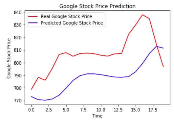
You are provided with a dataset consisting of stock prices for Google Inc, used to train a model and predict future stock prices as shown below.

For improved predictions, you can train this model on stock price data for more companies in the same sector, region, subsidiaries, etc. Sentiment analysis of the web, news, and social media may also be useful in your predictions. The open-source developer Sentdex has created a really useful tool for S&P 500 Sentiment Analysis.

Recurrent Neural Networks

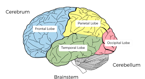
As we try to model Machine Learning to behave like brains, weights represent long-term memory in the Temporal Lobe. Recognition of patterns and images is done by the Occipital Lobe which works similar to Convolution Neural Networks. Recurrent Neural Networks are like short-term memory which remembers recent memory and can create context similar to the Frontal Lobe. The Parietal Lobe is responsible for spacial recognition like Botlzman Machines. Recurrent Neural Networks connect neurons to themselves through time, creating a feedback loop that preserves short-term and long-term memory awareness.

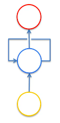
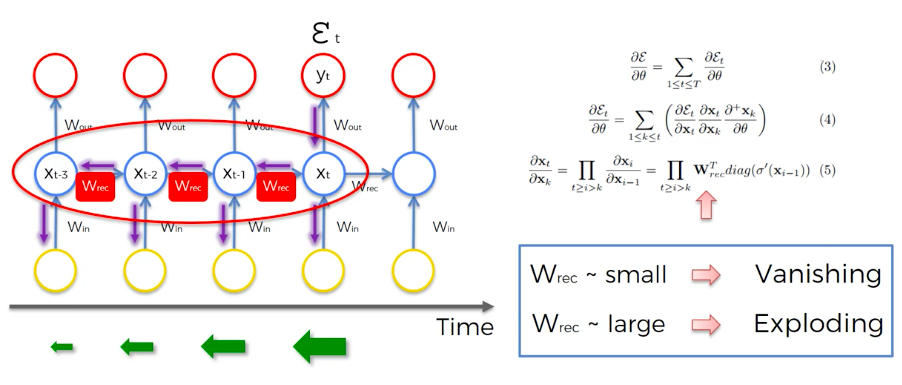
The following diagram represents the old-school way to describe RNNs, which shows a Feedback Loop (temporal loop) structure that connects hidden layers to themselves and the output layer which gives them a short-term memory.

Compact Form Representation

Expanded Form Representation

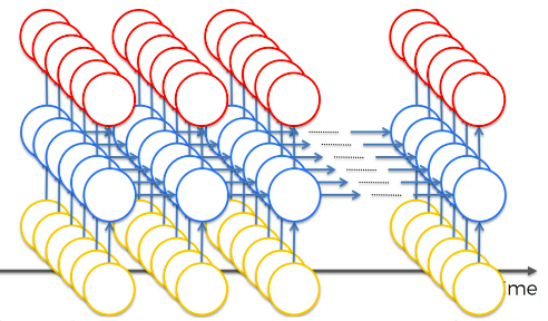
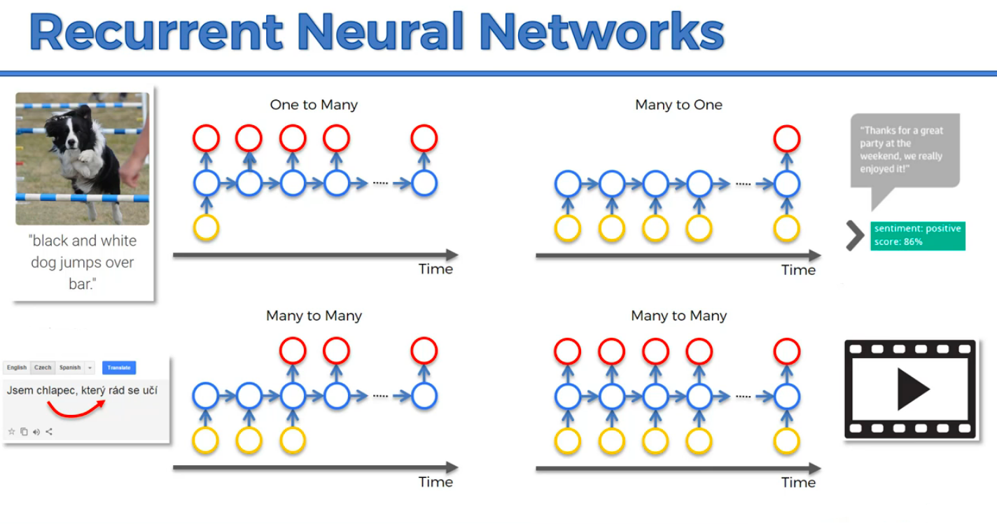
A more modern representation shows the following RNN types and use examples:

1. One-To-Many: Computer description of an image. CNN used to classify images and then RNN used to make sense of images and generate context.

2. Many-To-One: Sentiment Analysis of text (gague the positivity or negativity of text)

3. Many-to-Many: Google translate of language who's vocabulary changes based on the gender of the subject. Also subtitling of a movie.

Check out Andrej Karpathy's Blog (Director of AI at Tesla) on Github and Medium.

Here is the movie script writen by an AI trained with an LSTM Recurrent Neural Network: Sunspring by Benjamin the Artificial Intelligence.

RNN Gradient Problem (Expanding or Vanishing)

The gradient is used to update the weights in an RNN by looking back a certain number of user defined steps. The lower the gradient, the harder it is to update the weights (vanishing gradient) of nodes further back in time. Especially because previous layers are used as inputs for future layers. This means old neurons are training much slower that more current neurons. It's like a domino effect.

Expanding Gradient Solutions

1. Truncated Back-propagation

Stop back-propagation after a certain point (not an optimal because not updating all the weights). Better than doing nothing which can produce an irrelevant network.

2. Penalties

The gradient can be penalized and artificially reduced.

3. Gradient Clipping

A maximum limit for the gradient which stops it from rising more.

Vanishing Gradient Solutions

1. Weight Initialization

You can be smart about how you initialize weights to minimize the vanishing gradient problem.

2. Echo State Network

Designed to solve vanishing gradient problem. It's a recurrent neural network with a sparsely connected hidden layer (with typically 1% connectivity). The connectivity and weights of hidden neurons are fixed and randomly assigned.

3. Long Short-Term Memory Networks (LSTM)

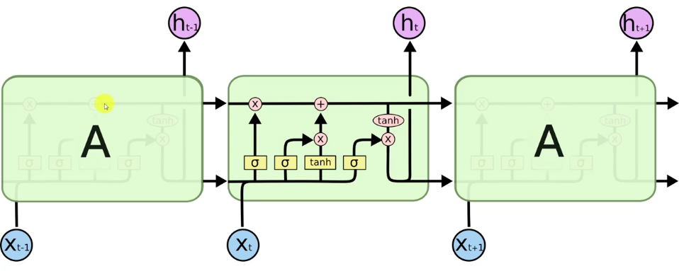
Most popular RNN structure to tackle this problem.

LSTM

When the weight of an RNN gradient 'W_rec' is less than 1 we get Vanishing Gradient, when 'W_rec' is more than 1 we get Expanding Gradient, thus we can set 'W_rec = 1'.

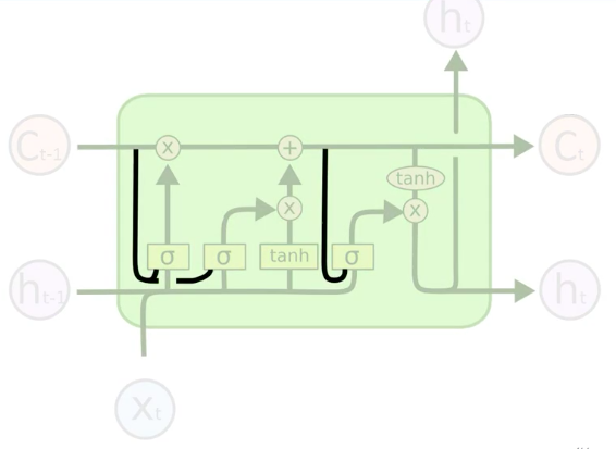
• Circles represent Layers (Vectors).

• 'C' represents Memory Cells Layers.

• 'h' represents Output Layers (Hidden States).

• 'X' represents Input Layers.

• Lines represent values being transferred.

• Concatenated lines represent pipelines running in parallel.

• Forks are when Data is copied.

• Pointwise Element-by-Element Operation (X) represents valves (from left-to-right: Forget Valve, Memory Valve, Output Valve).

• Valves can be open, closed or partially open as decided by an Activation Function.

• Pointwise Element-by-Element Operation (+) represent a Tee pipe joint, allowing stuff through if the corresponding valve is activated.

• Pointwise Element-by-Element Operation (Tanh) Tangent function that outputs (values between -1 to 1).

• Sigma Layer Operation Sigmoid Activation Function (values from 0 to 1).

LSTM Step 1

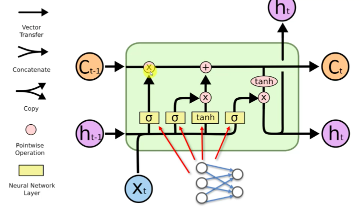
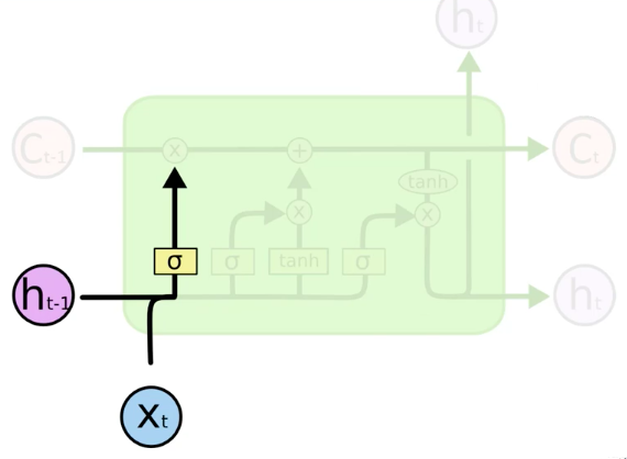
New Value 'X_t' and value from previous node 'h_t-1' decide if the forget valve should be opened or closed (Sigmoid).

LSTM Step 2

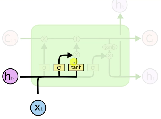
New Value 'X_t' and value from Previous Node 'h_t-1'. Together they decide if the memory valve should be opened or closed (Sigmoid). To what extent to let values through (Tanh from -1 to 1).

LSTM Step 3

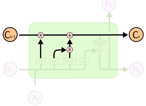
Decide the extent to which a memory cell 'C_t' should be updated from the previous memory cell 'C_t-1'. Forget and memory valves used to decide this. You can update memory completely, not at all or only partially.

LSTM Step 4

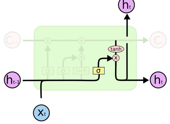
New value 'X_t' and value from previous node 'h_t-1' decides which part of the memory pipeline, and to what extent they will be used as an Output 'h_t'.

LSTM Variation 1 (Add Peep holes)

Sigmoid layer activation functions now have additional information about the current state of the Memory Cell. So valve decisions are made, taking into account memory cell state.

LSTM Variation 2 (Connect Forget & Memory Valves)

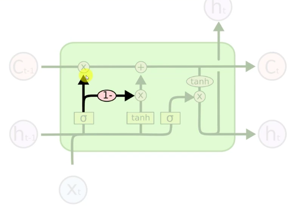
Forget and memory valves can make a combined decision. They're connected with a '-1' multiplier so one opens when the other closes.

LSTM Variation 3 (GRU: Gated Recurring Units)

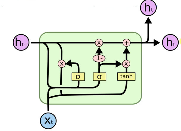
The memory pipeline is replaced by the hidden pipeline. Simpler but less flexible in terms of how many things are being monitored and controlled.

Code

Download the code and run it with 'Jupyter Notebook' or copy the code into the 'Spyder' IDE found in the Anaconda Distribution. 'Spyder' is similar to MATLAB, it allows you to step through the code and examine the 'Variable Explorer' to see exactly how the data is parsed and analyzed. Jupyter Notebook also offers a Jupyter Variable Explorer Extension which is quite useful for keeping track of variables.

$ git clone https://github.com/AMoazeni/Machine-Learning-Stock-Market-Prediction.git
$ cd Machine-Learning-Stock-Market-Prediction