What’s growing there?

Using eo-learn and fastai to identify crops from multi-spectral remote sensing data

A section of the Orange River, South Africa: colour imagery and NDVI from Sentinel 2 and target masks from Zindi’s Farm Pin Crop Detection Challenge

Introduction

This post describes how I used the eo-learn and fastai libraries to create a machine learning data pipeline that can classify crop types from satellite imagery. I used this pipeline to enter Zindi’s Farm Pin Crop Detection Challenge. I may not have won the contest but I learnt some great techniques for working with remote-sensing data which I detail in this post.

Here are the preprocessing steps I followed:

1. divided an area of interest into a grid of ‘patches’,

2. loaded imagery from disk,

3. masked out cloud cover,

4. added NDVI and euclidean norm features,

5. resampled the imagery to regular time intervals,

6. added raster layers with the targets and identifiers.

I reframed the problem of crop type classification as a semantic segmentation task and trained a U-Net with a ResNet50 encoder on multi-temporal multi-spectral data using image augmentation and mixup to prevent over-fitting.

My solution borrows heavily from the approach outlined by Matic Lubej in his three excellent posts on land cover classification with eo-learn.

The python notebooks I created can be found in this github repository: https://github.com/simongrest/farm-pin-crop-detection-challenge

The challenge

Zindi is an African competitive data science platform that focusses on using data science for social benefit. In Zindi’s 2019 Farm Pin Crop Detection Challenge, participants to **trained machine learning models using Sentinel2 imagery in order to classify the crops being grown in fields **along a stretch of the Orange River in South Africa.

The data supplied to contestants consisted of two shape files containing the training set and test set’s field boundaries, as well as Sentinel2 imagery for the area of interest at 11 different points in time between January and August 2017.

The section of the Orange River — grey test set fields interspersed amongst green training set fields

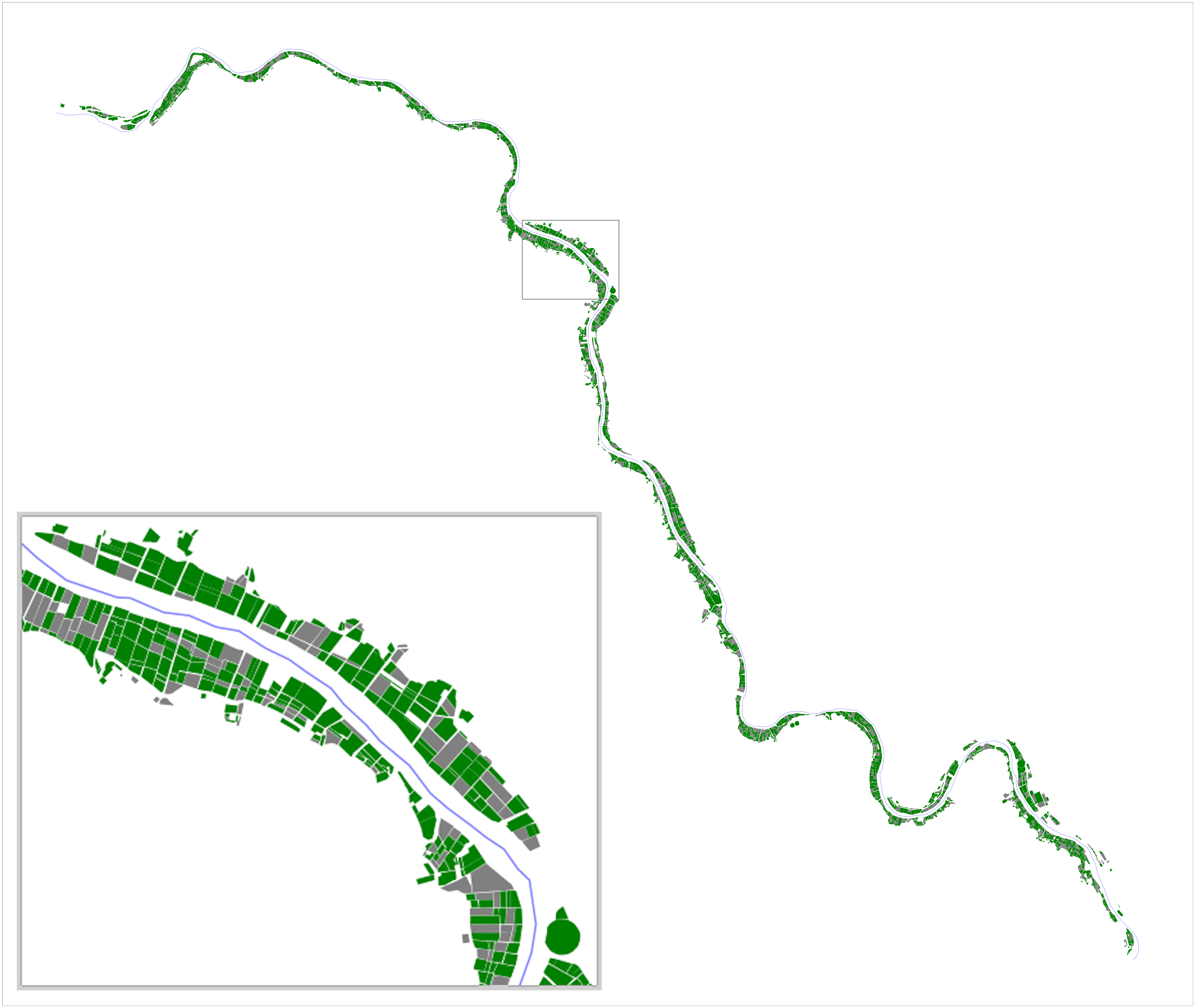
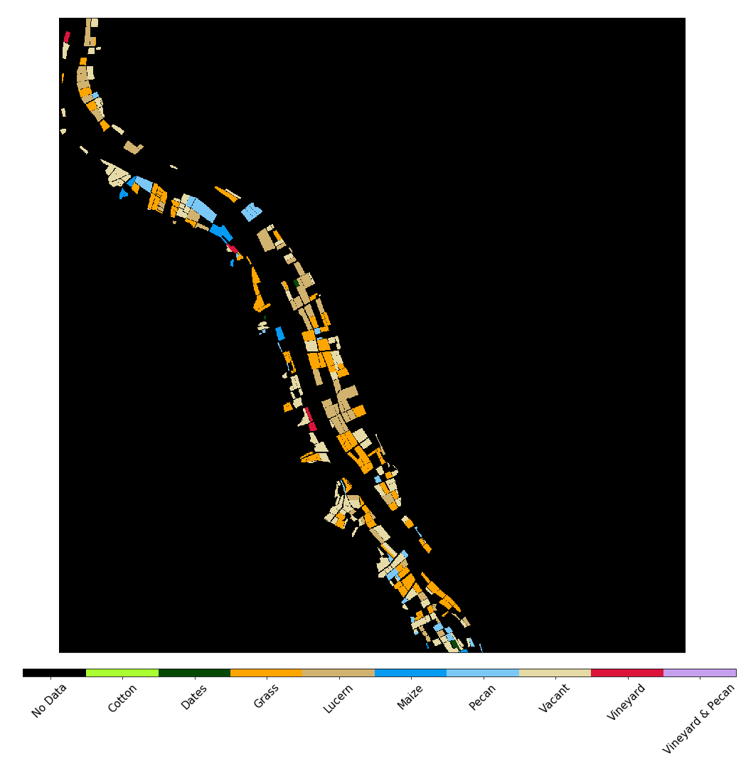
The training and test sets consisted of 2497 fields and 1074 fields respectively. Each field in the training set was labelled with one of nine labels indicating the crop that was grown in that field during 2017.

The crop types were:

Cotton
Dates
Grass
Lucern
Maize
Pecan
Vacant
Vineyard
Vineyard & Pecan (“Intercrop”)

Competitors were only to use the provided data and (due to a data leak discovered during the competition) were prohibited from using Field_Id as a training feature.

Data pre-processing with eo-learn (notebook)

The eo-learn library allows users to divide up an area of interest into patches, define a workflow and then execute the workflow on the patches in parallel.

1. Splitting the area of interest

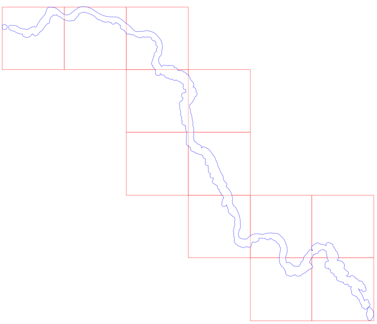
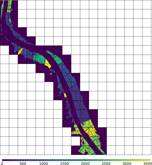
Using BBoxSplitter from the sentinelhub library I split the river up into 12 patches:

The area of interest partitioned into a grid of ‘patches’

2. Loading the image data from disk

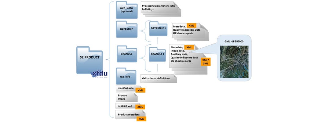
The image data for the competition was supplied in JPEG2000 format in the standard Sentinel2 folder structure illustrated below:

Sentinel2 folder structure

The eo-learn library has many useful predefined tasks for loading imagery from Sentinel Hub, manipulating imagery and generating features. At the time of writing it did not have a task to load imagery from disk in the format specified above. Nevertheless, defining my own EOTask class to do this proved simple enough. EOTask classes need an execute() method that optionally takes an EOPatch object as an argument.

EOPatch objects are essentially just collections of numpy arrays along with metadata. The EOPatch objects loaded by my own custom EOTask looked something like this:

data: {
    BANDS: numpy.ndarray(shape=(11, 1345, 1329, 13), dtype=float64)
  }
  mask: {}
  mask_timeless: {}
  scalar_timeless: {}
  label_timeless: {}
  vector_timeless: {}
  meta_info: {
    service_type: 'wcs'
    size_x: '10m'
    size_y: '10m'
  }
  bbox: BBox(((535329.7703788084, 6846758.109461494), (548617.0052632861, 6860214.913734847)), crs=EPSG:32734)
  timestamp: [datetime.datetime(2017, 1, 1, 8, 23, 32), ..., datetime.datetime(2017, 8, 19, 8, 20, 11)], length=11
)

We can visualise the patches by using bands 4, 3 and 2 (red, green and blue) to generate a colour image for each patch:

Colour images of the 12 patches made with the red, green and blue bands

3. Masking out clouds

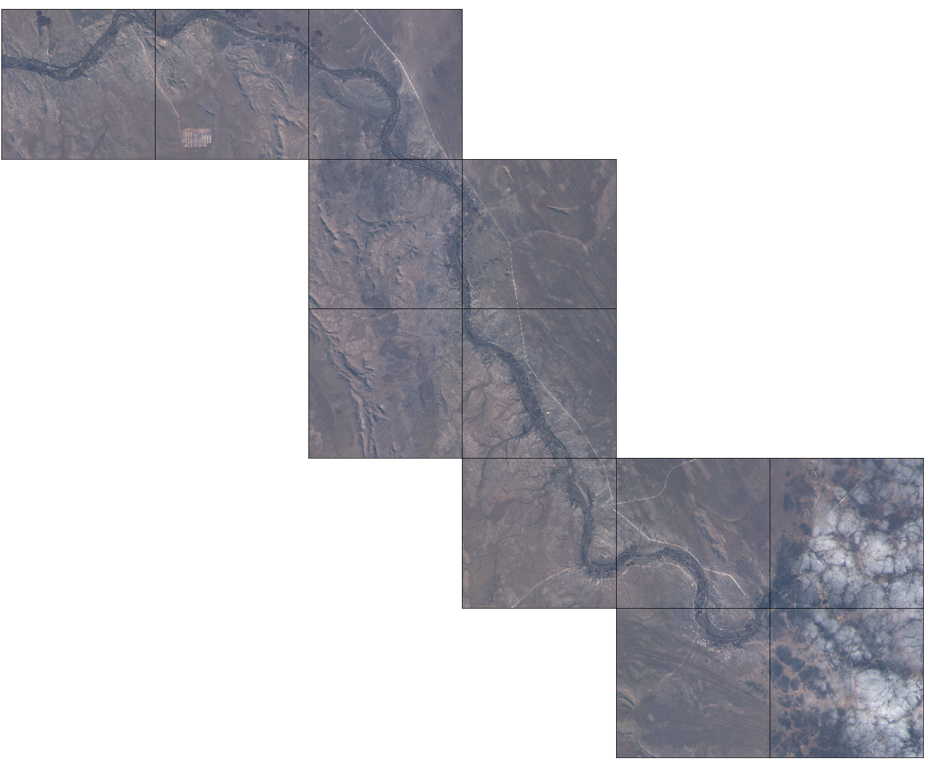
In the bottom right corner of the above image there is some cloud cover. The eo-learn library provides a pre-trained pixel-level cloud detector model. This functionality is available through the S2PixelCloudDetector* and *theAddCloudMaskTask classes.

The S2PixelCloudDetector comes from a separate library sentinel2-cloud-detector and uses all 13 bands of the Sentinel2 imagery to make its predictions. By setting a probability threshold the cloud probability predictions can be turned into a cloud mask.

Colour image with clouds, cloud probabilities and resulting cloud mask

I used this cloud detection functionality to add a cloud mask to my data.

4. Resampling through time

Cutting out clouds leaves gaps in the data for the areas with cloud cover in each time slice. One possible approach to filling these gaps is to interpolate between preceding and subsequent time slices.

There’s already a LinearInterpolation EOTask defined for this purpose. The class requires that you specify which bands to interpolate and an interval to resample on. I decided to average out my data to approximately one time slice per month, which reduced my time dimension from 11 time points to 8.

Additionally, to deal with any gaps at the start or end of the time period I used a ValueFilloutTask for simple extrapolation by copying values from preceding or succeeding time points as necessary.

5. Adding NDVI

*Normalized difference vegetation index *(NDVI) is a simple indicator of the presence of plant life in satellite imagery. The index is calculated using the red and near infra-red (NIR) bands.

NDVI = (NIR - Red)/(NIR + Red)

The Wikipedia article on NDVI has a nice explanation for the rationale behind this indicator. The essential idea is that plant matter absorbs much of visible red spectrum light while it reflects near infrared light which it cannot use for photosynthesis, NDVI captures this difference in reflectance in a ratio.

Conveniently eo-learn provides an NormalizedDifferenceIndex task which allowed me to easily compute and add NDVI for each of the patches.

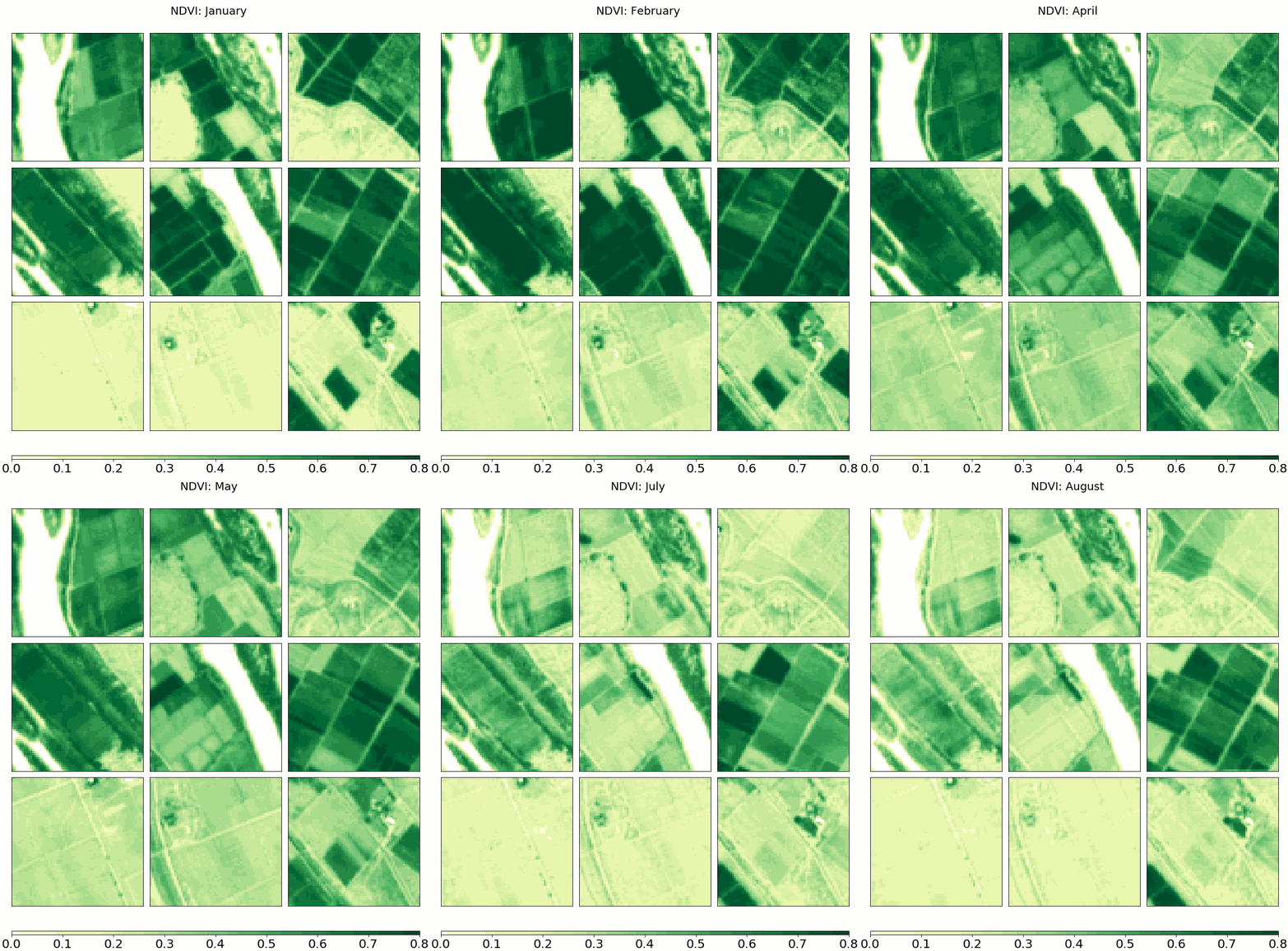
NDVI evolves differently through time for different crops. Different crops are planted and harvested at different times and grow at different rates. The animation below shows how NDVI evolves differently for adjacent fields.

NDVI through time (in March you can see artefacts that result from the cloud masking and interpolation)

6. Adding the target masks

In order to treat the crop identification challenge as a semantic segmentation task I needed to create target masks for our imagery. The VectorToRaster task in eo-learn takes vector geometries and creates a rasterised layer. I used this task to add a raster layer indicating the crop types. I also added a layer with the field identifiers for use in inference.

Crop type raster layer for patch number 6

Creating a workflow and executing it

To run each of the above preprocessing steps I put all the tasks into a workflow. In general, an eo-learn workflow can be any acyclic directed graph with EOTask objects at each node. I just used a linear workflow which looked something like:

LinearWorkflow(
 add_data,           # load the data
 add_clm,            # create cloud mask
 ndvi,               # compute ndvi
 norm,               # compute the euclidean norm of the bands
 concatenate         # add the ndvi and norm to the bands
 linear_interp,      # linear interpolation
 fill_extrapolate,   # extrapolation
 target_raster,      # add target masks
 field_id_raster,    # add field identifiers
 save                # save the data back to disk
)

To execute this workflow I created execution arguments for each patch and then used an EOExecutor to run the entire workflow on all of the patches in a distributed fashion.

execution_args = []
for patch_idx in range(12):
    execution_args.append({
        load: {'eopatch_folder': f'eopatch_{patch_idx}'},
        save: {'eopatch_folder': f'eopatch_{patch_idx}'}
    })
    
executor = EOExecutor(workflow, execution_args, save_logs=True)
executor.run(workers=6, multiprocess=False)

Building a prediction model

Semantic segmentation

Semantic segmentation is the process of assigning a class label to each pixel of an image. By reframing the crop identification problem in this challenge as a semantic segmentation task I could take advantage of the information in the local spatial context of each field, as I show below, it also allowed me to generate more training data by repeated sampling.

1. Generating the training set (notebook)

From my 12 patches I randomly sampled 64 x 64 pixel ‘patchlets’ to train my model. I kept the patch size small as the fields themselves are relatively small and the provided Sentinel2 imagery has a maximum spatial resolution of 10m . This means a square field 1 hectare in size (10,000m²) is appears in the imagery as an area of 32 x 32 pixels.

I sampled the patchlets in a manner that ensured that each patchlet contained at least a part of a training field. For each patchlet I saved two pickle files, one containing the input imagery and the other the raster layer with the crop types.

For the input imagery I chose to include six channels, the three visible bands (red, green and blue), near infra-red and the calculated NDVI and euclidean norm. When I resampled the imagery by interpolating through time I ended up with eight different time points. In order to get a rank three tensor, I simply stacked the six channels at each of the eight time points to get a 48-channel image.

NDVI and visible images at a single time point along with the corresponding target crop types for nine randomly sampled 64x64 training ‘patchlets’

2. Data augmentation

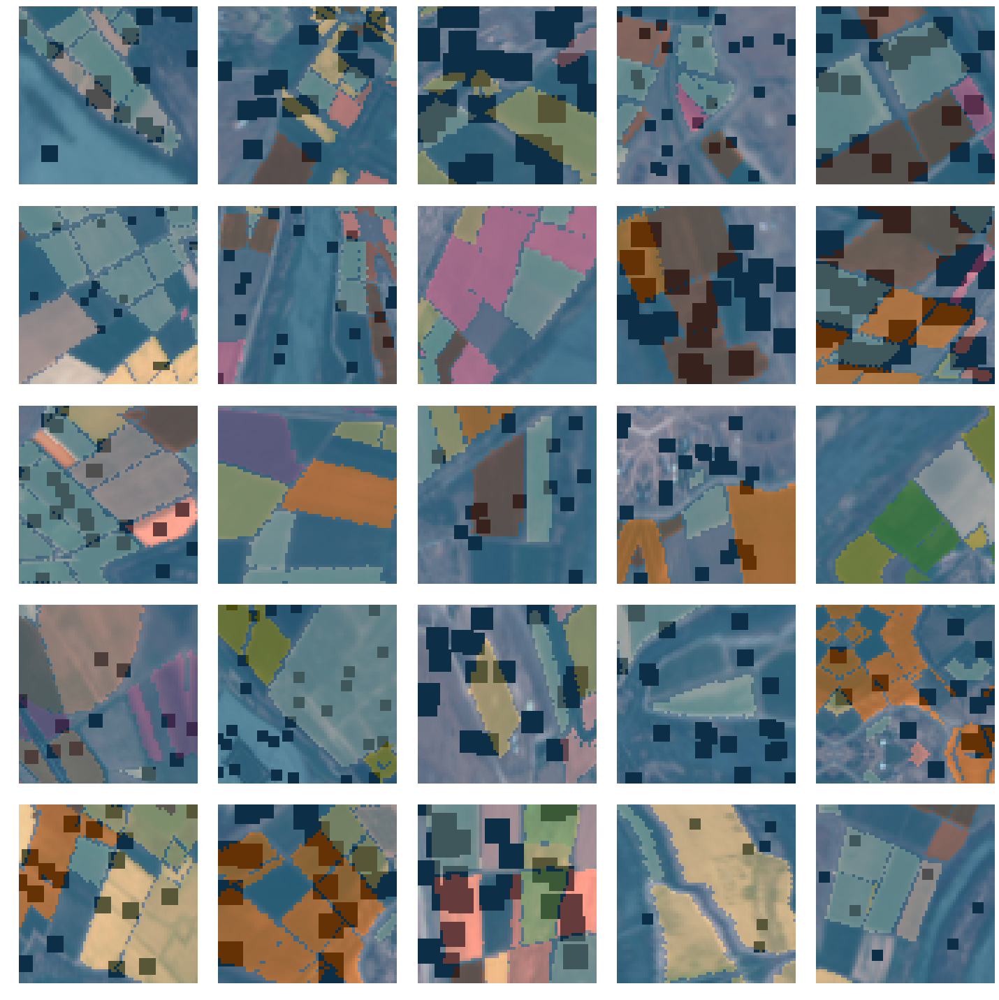
The relatively small dataset available in the competition and the large number of parameters in my chosen network architecture meant that I needed to be particularly careful of overfitting. To avoid this I use image augmentation as well as mixup.

The fastai library provides an array of image augmentation techniques. I used:

• vertical flips

• horizontal flips

• rotation

• zoom

• warping

• and cutout

A batch of training images with image augmentations applied

3. Creating a fastai U-Net model (notebook)

The fastai library provides for semantic segmentation by allowing the user to dynamically build a U-Net from an existing convolutional network encoder. I chose a ResNet50 pre-trained on ImageNet as my encoder network. To deal with the shape of my input tensors I replaced the first convolutional layer of the ResNet50 network that takes 3 channels with one that takes 48 channels instead.

I won’t attempt to explain U-Nets or residual neural networks here as there are many good explanations available already. For example here’s a post explaining U-Nets and here’s another explaining ResNets.

I created SegmentationPklList and classesSegmentationPklLabelList to implement functionality to load pickle file ‘images’ so that my data worked with the fastai’s data block API.

The fastai MixUpCallback and MixUpLoss also needed some minor tweaking to work with semantic segmentation.

4. Loss function

I used a modifiedCrossEntropyFlat loss function to score my model. I instantiated it as:

CrossEntropyFlat(axis=1, weight=inv_prop, ignore_index=0)

The occurrence of the different crop types in the training set was imbalanced, certain of the crop types only occurring a handful of times. I weighted my loss function in proportion with the inverse frequency of each crop type by using the weight parameter of the loss constructor.

Much of the area of the training images did not have a crop type, either there was no field in that region, or it if there was a field it was not part of the training set. I ignored predictions where there is no crop type label by using the ignore_index parameter of the loss constructor.

5. Training

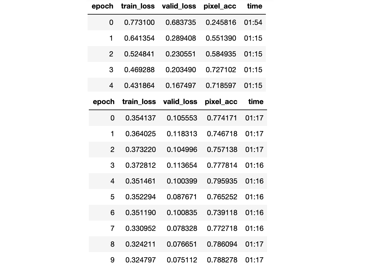
One of the biggest advantages that the fastai library offers is a flexible training loop along with great out of the box support for controlling training parameters through techniques such as the one cycle training policy. I trained my U-Net for five epochs using the fit_one_cycle function keeping the pre-trained encoder parameters frozen, and then for a further ten epochs allowing the encoder weights to be updated.

During training the loss on the validation set decreased consistently and my custom pixel accuracy metric increased fairly steadily.

Training results from 5 frozen and 10 unfrozen epochs

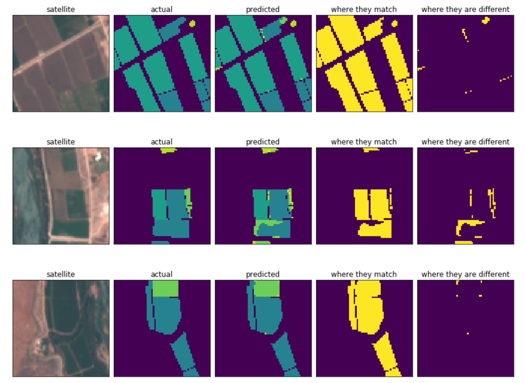
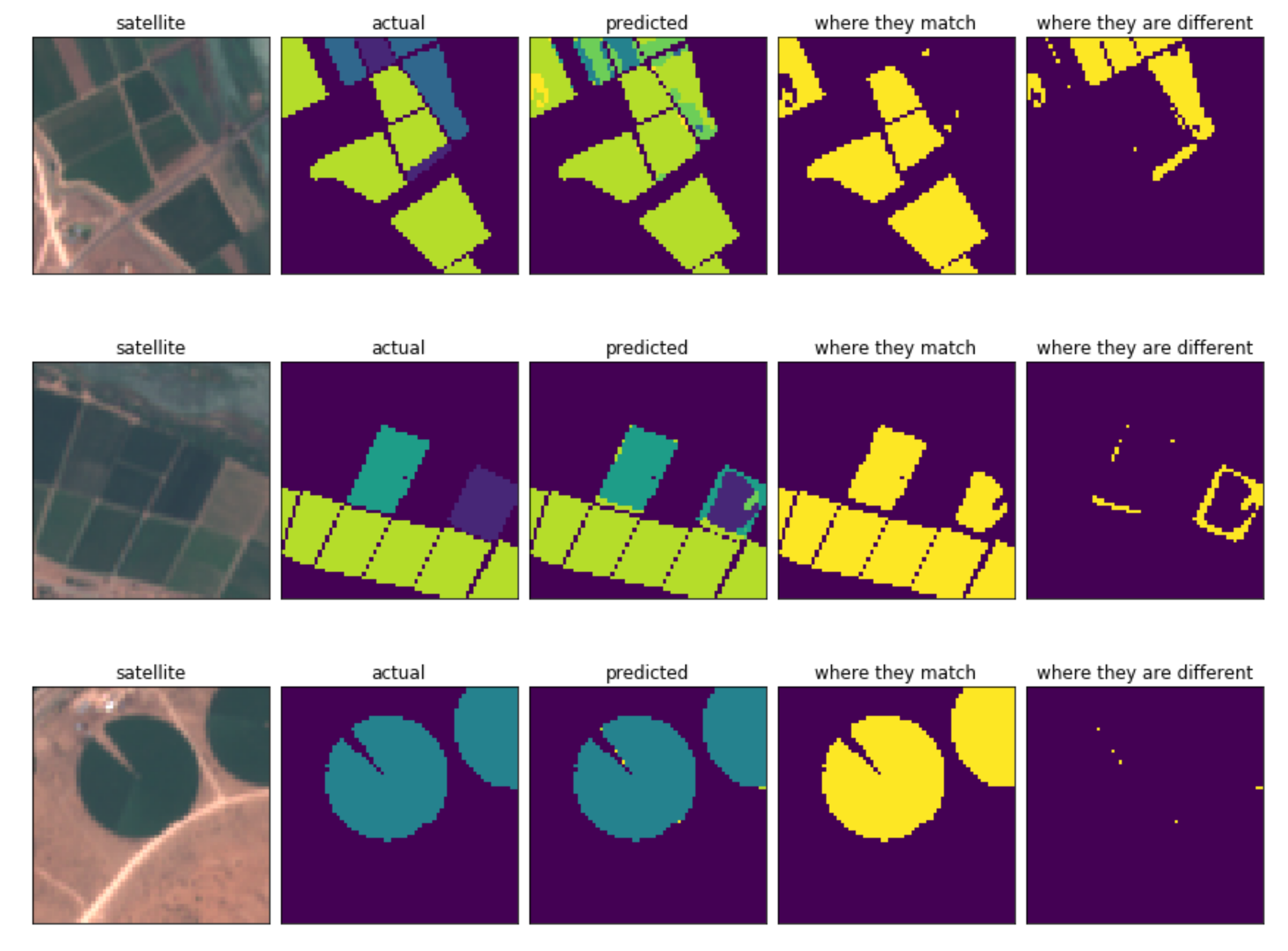
Comparing the predicted pixel masks to the target masks for examples in the validation set seemed to indicate that the network was working reasonably but that that there were examples of poor performance on the minority classes and fields with non-standard shapes.

More predictions on examples from the validation set

Results and areas for improvement

To do inference on the test set, I divided up each patch into a grid of 64x64 ‘patchlets’ and saved the pickle files for each patchlet. I made predictions for the entire test set and grouped the result by theField_Id. Predictions for each pixel consisted of the ten final activations from the U-Net. I took the median activation value for each class, and then applied a softmax function to get a single probability per crop for every Field_Id in the test set.

sample grid of ‘patchlets’ for inference — colouring by Field_Id clearly shows the data leak

Taking advantage of temporal patterns

Reflecting on my approach, I think that the area where the most improvement could have been made was in the treatment of the time dimension. My naive approach of stacking all the timepoints in 48 channels does not allow my model to properly learn from patterns in the imagery through time. I would have liked to explore using recurrent networks to learn these temporal patterns.

The team behind eo-learn have themselves have proposed using a Temporal Fully-Convolutional Network (TFCN) for this: https://sentinel-hub.com/sites/default/lps_2019_eolearn_TFCN.pdf. TFCNs take rank 4 tensors as inputs and use 3D convolutions to capture patterns in space and time simultaneously.

Building latent representations using unsupervised learning

If the competition had allowed for the use of external data, it would have been interesting to explore the Tile2Vec technique described in this paper https://arxiv.org/abs/1805.02855. The idea here is to generate latent vector representations of areas from satellite imagery by setting up an unsupervised learning task using a triplet loss.

I am very curious to learn what approaches the other competitors employed.

Thanks

I’d like to thank the team at Zindi for putting together such an interesting challenge. I’d also like to thank the eo-learn team both for providing such a useful library and for such engaging posts on how to use it. Thanks too to the fastai community for all their work in making deep learning more approachable and broadly accessible. Finally I’d like to thank Stefano Giomo for all his input on this project.

Copyright and attribution

The code in the notebooks in this repository is licensed under the Apache Licence, Version 2.0. Please feel free to modify and re-use it. If you find this work useful and re-use it in a public context it would be great if you could mention where the code originated.